Data Manipulation: SQL Vs R
 By: Kunal Gera
Introduction using SQL in R
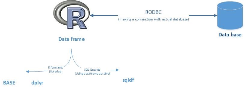
The two part of it,
- Using data frame as table (as database table)
- Using base function (other library ‘dplyr’)
- Using ‘sqldf’
- Connecting with actual database
I will be explaining the former one.
Using data frame as table
SQL data manipulation task
- Select with ‘where’, ‘group by’ and ‘order by’ clause
- Count with ‘where’ clause
- Join
- Update
- Addition of column
- Applying function
A.Using base function
[I will be giving code snippets of the above mentioned function in ‘base’]
Increasing efficiency of base code using ‘data.table’ library. This library is also
There is other library in R for DML, it is ‘dplyr’. [I will not be explaining it]
B.Introduction to SQL Library in R (‘sqldf’)
[I will be giving code snippets of the above mentioned function in ‘sqldf’]
SQL in R
Data! Data! Data, here, there and now everywhere. We are generating data from most of the activity we perform these days. From buying grocery to buying a car, from sleeping with an alarm to gyming.
To handle this amount of data we need tools to manipulate it efficiently. As we can’t consume raw food similarly we can’t consume raw data. We need to cook it, and for that we have a great tools.
This article is specifically very useful for learners who know SQL and want to explore R.
Prerequisite:
Skills
- Knowledge of SQL
- Basic knowledge of R and data frames (You can think ‘data frames’ as ‘table’ in a database).
Software
- Any R IDE.
- Any Database (For connecting to real database)
Introduction to SQL in R
SQL is a very powerful language for talking to any relational database. This power can be multiplied when clubbed with R. R is a statistical software which is highly used in data mining and analytics industry. As it is an open source software, it turns to be a great choice for many.
R is been used in various task ranging from analytical model building, visualising the data to even report generation. To start in R we need to learn few basic of data manipulation, as a SQL user you must have performed many query based manipulation. Let’s now learn how we can do the same in R.
Today, we will be focusing on how we can make R talk and understand SQL and getting the same result as we get from SQL in database.
We will be learn most used data manipulation techniques, for that we will cover following topics:
| S. No. | SQL | R |
| A | Where clause | Subset |
| B | Group by clause | Aggregate |
| C | Order by | Sort & Aggrange |
| D | Transforming a column | Mutate & tranformation |
| E | Distinct | Duplicated |
| F | Join | Merge |
Making R behave and understand SQL
We will be applying function and queries on dataframes in R
- Base & ‘dplyr’ Function (Using R functions to give output similar to SQL)
- Sqldf package (Using SQL queries on dataframe)
Making R speak SQL
- Connect R with actual database
Let’s start cooking
For cooking the data we will need two things:
A. R Libraries (spice)
Base, ‘dplyr’ and Sqldf’ (SQLite queries)
- Base is available
- library(dplyr)
- library(sqldf)
We will be learning the functions in each library to get the same output.
B. Data (raw food)
For today’s learning we will be using ‘airquality’ dataset in R, which we can load the dataset by following command:
Loading the dataset
data(airquality)
Let’s now understand (seeing the datatype, base statistics and first few rows) about the dataset by using the important commands in R
Understanding the dataset
str() can used to know the datatype and few observation of any dataframe.
str(airquality)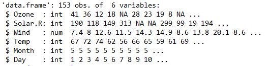 Similarly, summary() can used to know the statistical details about the observation of any dataframe. Eg: Mean, Median, Quartiles and frequency and etc.
summary(airquality)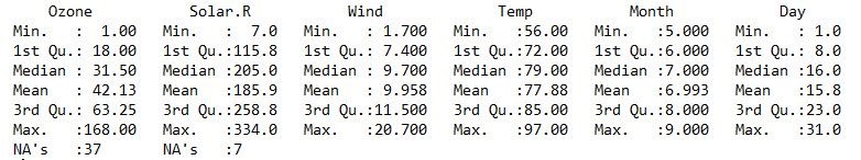 head() is an easy and quick way to look few row of any dataframe.
head(airquality)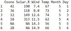 dim() is a function to know the dimension any dataframe i.e. count of rows and column.
dim(airquality)
[1] 153 6
| Quick Tip: You can write ‘?functionname‘ in R console to know more about that function. E.g. ‘dim‘ will show the documentation on ‘dim()’ function. |
So, airquality is data of daily air quality measurements in New York, from May to September 1973.
Ozone numeric Ozone (ppb)
Solar.R numeric Solar R (lang)
Wind numeric Wind (mph)
Temp numeric Temperature (degrees F)
Month numeric Month (1–12)
Day numeric Day of month (1–31)
Hope you guys have understood the ‘airquality’ dataset, it not that tough though.
So now, we know our data set so we can start cooking our dataset with the above mentioned technique and functions.
A. Subset
It is simple to understand and most useful technique in data manipulation, i.e. subset: which is filtering the data set based of some condition or clause.
Base
“Subset in BASE“: subset(airquality, Month == 5)
OR
airquality[airquality$Month == 5,]
Selecting specific columns: So, if we want Ozone,Solar.R, Month and Temp from airqualit then following command can be used:
airquality[,c(“Ozone”,”Solar.R”,“Month”,”Temp”)]
dplyr
“filter in dplyr”: filter(airquality,Month == 5)
“Selecting specific columns”:
select(airquality,Ozone,Solar.R,Month,Temp)
Note: We can use pipes(%>%) to make it one command
airquality %>% filter(Month==5) %>% select(Ozone,Solar.R,Month,Temp)
Pipe consider the left side dataframe for right side function which is similar to SQL.
sqldf
“Where clause in sqldf”: sqldf(‘Select * from airquality where Month = 5; ‘)
“Selecting specific columns “: sqldf(‘Select Ozone,Solar.R,Month,Temp from airquality where Month = 5; ‘)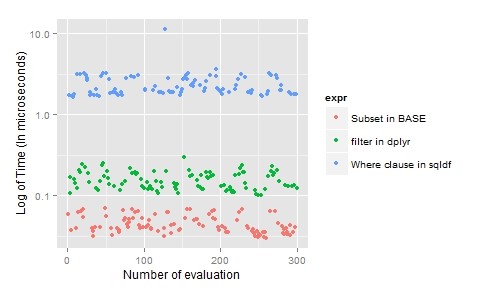
For subset in R, “base” is preferred as it is laconic and time efficient.
B. Aggregate
It is highly used technique in data manipulation, summarising or aggregating (i.e. sum, mean, standard deviation etc.) the data on a grouping variable.
Here, we will find the sum of Temp and average of Wind grouped by Month.
Base
aggregate(airquality[,c(TotalTemp = “Temp”,”Wind”)], list(“Month” = Month),mean)
OR
aggregate(cbind(“AverageTemp” = airquality$Temp, “AverageWind” = airquality$Wind) ~ Month, data = airquality, FUN=mean)
Note: We can’t apply two or more aggregate functions on different columns, but we can apply one function to all the columns. So we have to re-apply the function accordingly.
dplyr
airquality %>% group_by(Month) %>%
summarise(“TotalTemp” = sum(Temp), “AverageWind” =
mean(Wind,2))
sqldf
sqldf(“select Month, sum(Temp) as TotalTemp, avg(Wind) as AverageWind from airquality group by Month;”)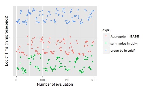
For aggregation, the choice is dplyr as it allows use of multiple aggregate function simultaneously, ease to understand and time-efficient.
C. Sort
Arranging or sort is a normal task used on various occasion in data manipulation, here we are sorting the data by ascending order of Month and descending order of Day.
Base
airquality_sorted_base <- airquality[order(airquality$Month,-airquality$Day),]
dplyr
airquality %>% arrange(Month,desc(Day))
sqldf
sqldf(“select * from airquality order by Month,Day desc;”)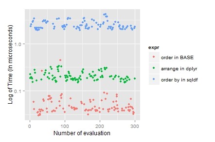
Usually the sorting data is combine with other data manipulation techniques, so “dplyr” become the first choice because it’s laconic and it can be clubbed using pipes.
D. Formulate a new column (transforming columns)
In manipulation of data, this may be an important task we need to perform sometimes. Assuming, we want to find out the Temp as percentage of total temperature of all months.
Base
airquality$TempPercentage <- airquality$Temp/(sum(airquality$Temp))
dplyr
airquality <- mutate(airquality, TempPercentage = Temp/sum(Temp))
sqldf
sqldf(“select aq.*,cast(Temp as real)/(select sum(Temp) from airquality) as TempPercentage from airquality aq;”)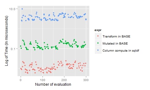
For transformation, “dpylr” is preferred as you can transform multiple column in single line of code but if you have only one or two columns you can use “base”.
E. Removing Duplicate (Single & multiple columns)
For removing duplicates you need a dataset with duplicate observation, for this we can use rbind() function to duplicate the current dataset by following command.
airquality_duplicated <- rbind(airquality,airquality)
Base
airquality_duplicated[!duplicated(airquality_duplicated[,c(“Month”,”Day”)]),]
dplyr
distinct_aq_dplyr <- airquality_duplicated %>% distinct(Month,Day)
sqldf
sqldf(‘select * from airquality_duplicated
where rowid in
(select min(rowid) from airquality_duplicated group by Month, Day)
;’)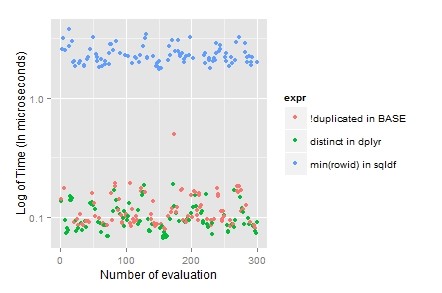
For removing duplicate, clearing “dpylr” is the choice because it’s laconic and easy to understand.
F. Join
Now, assuming we want to add “Month” name in the dataset, we can do this by various method, one of which is using join or merging technique. For this, just create a file named “monthnames.csv” with the below values and import the file in R environment as ‘monthnames’ (dataframe)
“1 Jan”
“2 Feb”
“3 Mar”
“4 Apr”
“5 May”
“6 Jun”
“7 Jul”
“8 Aug”
“9 Sep”
“10 Oct”
“11 Nov”
“12 Dec”
To import the file, save the above file in your working directory and run the following command
monthnames <- read.csv(file = “monthnames.csv”, header=FALSE)
names(monthnames) = c(“Month”,”MonthName”)
Base
airquality_join_base <- merge(x = airquality, y = monthnames, by.x = “Month”, by.y = “Month”, x.all=TRUE)
Similarly,
Outer join: merge(x = airquality, y = monthnames, by.x = “Month”, by.y = “Month”, all = TRUE)
Left outer: merge(x = airquality, y = monthnames, by.x = “Month”, by.y = “Month”, all.x = TRUE)
Right outer: merge(x = airquality, y = monthnames, by.x = “Month”, by.y = “Month”, all.y = TRUE)
dplyr
airquality_join_dplyr <- inner_join(x = airquality, y = monthnames, by = c(“Month” = “Month”))
Similarly,
Outer join: full_join(x = airquality, y = monthnames, by = c(“Month” = “Month”))
Left outer: left_join(x = airquality, y = monthnames, by = c(“Month” = “Month”))
Right outer: right_join(x = airquality, y = monthnames, by = c(“Month” = “Month”))
sqldf
airquality_sqldf <- sqldf(‘select aq.*,mn.MonthName from airquality aq
inner join monthnames mn
on aq.Month = mn.Month; ‘)
Similarly,
Left join: sqldf(‘select aq.*, mn.MonthName from airquality aq
left join monthnames mn
on aq.Month = mn.Month;’)
Note: RIGHT and FULL OUTER JOINs are not currently supported in sqldf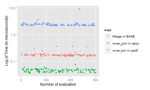
For joins, “dplyr” is the clearly the best as it’s laconic, time-efficient and easy to understand.
Conclusion
| S. No | Topic | Utility | BASE | dplyr | sqldf |
| A | Subset | Very frequent | 1 | 2 | 3 |
| B | Aggregate | Frequent | 2 | 1 | 3 |
| C | Sort | Very frequent | 1 | 2 | 3 |
| D | Transform | Less frequent | 1 | 2 | 3 |
| E | Duplicate | Very frequent | 1 | 1 | 3 |
| F | Join | Frequent | 2 | 1 | 3 |
| Total (Least the better) | 8 | 9 | 18 | ||
*Least the better
There is a minute difference in time for ‘base’ and ‘dplyr’, though ‘base’ is a clear winner but I suggest to choice a ‘dplyr’ package based on following reasons:
- Substantially efficient on big size dataset
- Capable of both in and out memory operation (i.e. dataframe and connect with database).
- Laconic and ease to understand.
- Connect R with actual database using ‘RODBC’
Step a) Create DSN Name for your database.
I will not be concentrating on this a lot on this, but at macros level, I will explain that it requires ODBC driver specific to database. You can google to find “How to setup ODBC connection”.
You can follow these articles to setup DSN name:
Step b) Connecting Database through R.
To connect any database through R we need a library called ‘RODBC’
library(RODBC)
i) Creating a connection with database, for that we will use odbcConnect() function in RODBC library.
db <- odbcConnect(dsn=”TEST “, uid=”USERNAME”, pwd=”PASSWORD”, believeNRows=FALSE)
Note: In oracle the username and password will be specific to the schema you want to connect.
ii) Importing data using SQL query through database connection, we will use sqlQuery() function in RODBC library.
DataFrame = sqlQuery(db, “Select * from TABLE”)
This have create a ‘dataframe’ with all observation in TABLE. You can now use the connection to perform any SQL query and import any table.
It is very powerful as the queries are performed by SQL in database and not R, but remember the data is getting transferred, between R and Database, every time you execute the query.
You can learn more on the above topics:
http://cran.r-project.org/web/packages/dplyr/
http://cran.r-project.org/web/packages/sqldf/
http://cran.r-project.org/web/packages/RODBC/
Author: Kunal Gera
Profile: Kunal has a strong background of finance and banking acumen.
He has been involved in requirement gathering and solving problem with the help of data analysis. He is well versed with various analytical concepts and have been using techniques like Logistic Regression, Tree, CART Model, Linear optimization, Integer optimization etc in his career.


kunalgera1 Posts
0 Comments